6 - Developing expectations for the future

Here we take a stab at establishing some capital market expectations with regression

In a recent note, I talked about valuations and the importance that they play in explaining future returns. Today, we’re going to approach developing these expectations in a more empirical way with linear regression. This will be the first note documeting my continued effort on this. The overall goal is to see if we can predict the 10 year expected real return on the S&P 500 based on metrics that measure the economy today.

Independent variables

I’m going to start by pulling in the total return CAPE ratio because we already know this explains some large share of the future 10 year realized returns on the S&P 500. “Total return” just refers to the fact that it includes dividends in the price, as opposed to the “price return” which doesn’t include dividends. I’m also going to include the US 10-year treasury rate minus the 2-year treasury rate. This is a powerful predictor of recessions because when the Federal reserve raises interest rates, this increases the 2-year yield faster than the 10-year yield, making the 2 year larger than the 10 year and therefore sending the 10yr - 2yr into negative territory. This is because, in some sense, the Fed induces recessions in order to slow down the economy when inflation gets high. You can see how this time series goes negative when a recession is on the horizon.

I am also incorporating the effective federal funds rate to get a sense of what the base cost of money is, which changes when the Federal reserve adjusts interest rates. Additionally, I include the unemployment rate, the rate on average 30 year mortgages, and the Chicago Fed National Financial Conditions Index which measures how tight or loose economic conditions are in equity and debt markets. These will be included, along with a few other popular measures of the US economy.

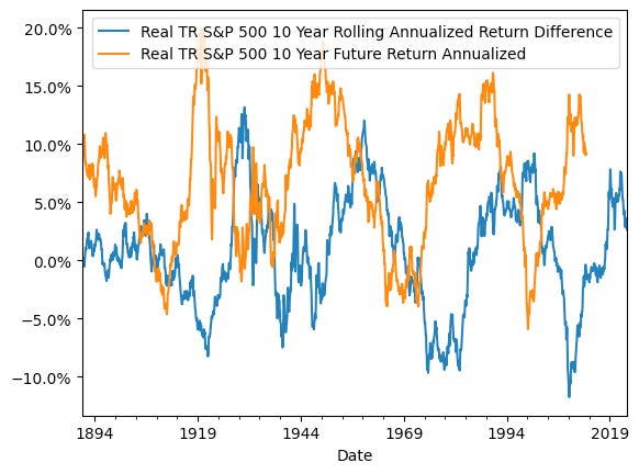
Mean reverting returns

I have been considering tracking how cumulative returns for the S&P 500 stray from the overall cumulative return. You can think about this as “what would the historical annualized return be if I invested in the S&P 500 in 1881” compared to “what has the annualized historical return been over the last 10 years”. This hinges on the idea that when recent returns have been higher than long run returns, future returns are likely to be lower. Below, you can see that the cumulative average return (in orange) is pretty stable, right around 5%, but the rolling 10 year annualized return is almost cyclical.

The chart below shows that when the past-10 year real return on the S&P 500 is higher than the total cumulative return, the next 10 years typically shows lower returns. We will evaluate this relationship later on.

Statistical significance

Now let’s take a look at the p values for all of the independent variables against the dependent variable to determine their statistical significance. The dependent variable in this case is the future 10 year annualized S&P 500 return. I also eliminate all values before 1976 because we need non-null variables and many of the independent variables from FRED only go back to 1976. In the back of my mind, I’m going to note that since the ‘70s we have really only seen interest rates fall until they reached rock bottom in 2009 when the Federal reserve tried to stimulate the economy as much as they could by lowering them to 0. 

Interestingly, the 10 year minus 2 year is the only one that has a p-value greater than 0.01. In this case, I’m going to eliminate it from the analysis and keep the rest.

Independent variable correlation

Next, we’re going to look at the absolute value correlation matrix.

You’ll notice that many of these independent variables are correlated with each other. This is called multicollinearity and it breaks a fundamental assumption of linear regression, which is that observations must be independent of each other. We will attempt to correct this later.

Skew

Another good thing to do is to check out the histogram of the dependent variable as I’ve done below.

As you can see, skew is present. This means that in our dataset, since the 1970s, the next 10 years tended to return more than 5% in real terms. This means our dataset is unbalanced. Ideally, we would see a normal distribution of values, and if it isn’t normal we could make transformations to force normality. For now, we’re going to leave this as is.

Regression

Next up, we’re going to pass our independent variables through a scaler. This scaler converts all values to their Z-score. A Z-score expresses how far away from the mean the value is. I’m doing this so I can pass these independent variables into a principle component analysis. You’ll recall that many of my independent variables expressed high correlations with each other, which is a problem. Principal component analysis decomposes and combines our old independent variables into new, uncorrelated, independent variables. Removing multicollinearity is a major advantage, but the catch is that we lose which old variables make up the new variables. Here is the correlation now, but notice that the variables are just labeled by their number, and the connection to the old variables is gone now.  

Now, we’re going to take our first stab at figuring out how predictive we can be with linear regression. This will be our baseline going forward. One thing I’ll note, is that I controlled for heteroskedasticity. This term refers to how the variance of residuals changes over time. If the variance is constant, then it is homoskedastic which is a requirement of linear regression. Most financial series are heteroskedastic like this one, so I have adjusted for that. I am also going to train the regression on the first 80% of the data, and then test the last 20% to see how good this regression is at predicting future returns. It can be misleading to just look at the adjusted R-squared since this represents how closely we can fit a line to all data that we have already seen, but it doesn’t tell us much about how the model is at predicting based on new data.

A couple other things to note

The Jarque-Bera value of 10.845 is pretty far from 0 with a p-value of 0.0042 indicating that this data is not normally distributed, which confirms what we already knew. It’s also worth noting that our residuals include auto-correlation. Auto-correlation is when the past value or values are correlated with future values. The Durbin Watson statistic only goes from 0 to 4, where 2 indicates no auto-correlation. Less than 2 indicates negative autocorrelation. All of this points to multiple linear regression not working for this type of data. Next, we will explore our other options.